Happy Thanksgiving 2022!!!

                     

Thanksgiving is a joyous invitation to shower the world with love and gratitude. Forever on Thanksgiving the heart will find the pathway home. The more you practice the art of thankfulness.

                   Wish you a very happy and blessed Thanksgiving!

Lupine Publishers| What is Quantum Computing and How it Works, Artificial Intelligence Driven by Quantum Computing

 Lupine Publishers| Modern Approaches on Material Science

What is Quantum Computing and How it Works, Artificial Intelligence Driven by Quantum Computing

Abstract

Companies such as Intel as a pioneer in chip design for computing are pushing the edge of computing from its present Classical Computing generation to the next generation of Quantum Computing. Along the side of Intel corporation, companies such as IBM, Microsoft, and Google are also playing in this domain. The race is on to build the world’s first meaningful quantum computer-one that can deliver the technology’s long-promised ability to help scientists do things like develop miraculous new materials, encrypt data with near-perfect security and accurately predict how Earth’s climate will change. Such a machine is likely more than a decade away, but IBM, Microsoft, Google, Intel, and other tech heavyweights breathlessly tout each tiny, incremental step along the way. Most of these milestones involve packing more quantum bits, or qubits-the basic unit of information in a quantum computer-onto a processor chip ever. But the path to quantum computing involves far more than wrangling subatomic particles. Such computing capabilities are opening a new area into dealing with the massive sheer volume of structured and unstructured data in the form of Big Data, is an excellent augmentation to Artificial Intelligence (AI) and would allow it to thrive to its next generation of Super Artificial Intelligence (SAI) in the near-term time frame.

Keywords: Quantum Computing and Computer, Classical Computing and Computer, Artificial Intelligence, Machine Learning, Deep Learning, Fuzzy Logic, Resilience System, Forecasting and Related Paradigm, Big Data, Commercial and Urban Demand for Electricity

Introduction

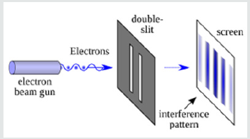
Quantum Computing (QC) is designed and structured around the usage of Quantum Mechanical (QM) concepts and phenomena such as superposition and entanglement to perform computation. Computers that perform quantum computation are known as Quantum Computers[1-5].Note that the superposition from a quantum point of view is a fundamental principle of quantum mechanics. The Quantum Superposition (QS) states that, much like waves in Classical Mechanics (CM) or Classical Physics (CP), any two or more quantum states can be added together (“superposed”), and the result will be another valid quantum state; and conversely, that every quantum state can be represented as a sum of two or more other distinct countries.Mathematically, it refers to a property of solutions to the both Schrödinger Time-Dependent and Time-Independent Wave Equations; since the Schrödinger equation is linear, any linear combination of solutions will also be a solution.An example of a physically observable manifestation of the wave nature of quantum systems is the interference peaks from an electron beam in a double-slit experiment, as illustrated in (Figure 1).The pattern is very similar to the one obtained by the diffraction of classical waves. [6]. Quantum computers are believed to be able to solve some computational issues, such as integer factorization, which underlies RSA encryption [7], significantly faster than classical computers. The study of quantum computing is a subfield of quantum information science.

Figure 1: Double-Slit Experiment Setup.

Historically, Classical Computer (CC) technology, as we know them from the past few decades to present, has involved a sequence of changes from one type of physical realization to another, and they have been evolved from main-frame of the old generation to generation of macro-computer. Now, these days, pretty much everyone owns a minicomputer in the form of a laptop, and you find these generations of computers in everyone’s house as part of their household. These mini-computers, Cemeterial Processing Units (CPUs), are based on transistors that are architected around Positive-Negative-Positive (PNP) junction.From gear to relays to valves to transistors to integrated circuits and so on we need automation and consequently augmentation of computer of some sort Today’s advanced lithographic techniques at below sub-micron innovative structure augmenting techniques such as Physical Vapor Deposition (PVD), Chemical Vapor Deposition (CVD), and Chemical Mechanical Polishing (CMP) can create chips with a feature only a fraction of micron wide. Fabricator and manufacturer these chips are pushing them to yield even smaller parts and inevitably reach a point where logic gates are so small that they are made out of only a handful of atoms size, as it is depicted in (Figure 2).

Figure 2: Today’s Chip Fabrication.

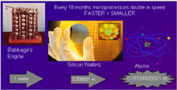
It worth mentioning that the size of the chip going way beyond sub-micron technology is limited by the wavelength of the light that is used in the lithographic technique.
On the atomic scale, matter obeys the rules of Quantum Mechanics (QM), which are quite different from Classical Mechanics (CM) or Physics Rules that determine the properties of conventional logic gates. Thus, if computers are to become smaller in the future, new, quantum technology must replace or supplement what we have new as a traditional way of computing.The point is, however, that quantum technology can offer much more than cramming more and more bits onto silicon CPU chip and multiplying the clock-speed of these traditional microprocessors. It can support an entirely new kind of computation with qualitatively new algorithms based on quantum principles! In a nutshell, in Quantum Computing, we deal with Qubits, while in Classical Computing, we deal with bits of information; thus, we need to understand “What Are Qubits?” and how it is defined, which we have presented this matter further down.Next generation of tomorrow’s computer is working based on where “Quantum Bits Compressed for the First Time.” The physicist has now shown how to encode three quantum bits, the kind of data that might be used in this new generation of computer, by just using two photons.Of course, a quantum computer is more than just its processor. These next-generation systems will also need new algorithms, software, interconnects, and several other yet-tobe- invented technologies specifically designed to take advantage of the system’s tremendous processing power-as well as allow the computer’s results to be shared or stored.

Intel introduced a 49-qubit processor code-named “Tangle Lake.” A few years ago, the company created a virtual-testing environment for quantum-computing software; it leverages the powerful “Stampede” supercomputer at The University of Texas at Austin to simulate up to a 42-qubit processor. To understand how to write software for quantum computers, however, they will need to be able to simulate hundreds or even thousands of qubits.Note that: Stampede was one of the most potent and significant supercomputers in the U.S. for open science research. Able to perform nearly ten quadrillion operations per second, Stampede offered opportunities for computational science and technology, ranging from highly parallel algorithms, highthroughput computing, scalable visualization, and next-generation programming languages, as illustrated in (Figure3) here. [8]This Dell PowerEdge cluster equipped with Intel Xeon Phi coprocessors pushed the envelope of computational capabilities, enabling breakthroughs never before imagined. Stampede was funded by the National Science Foundation (NSF) through award ACI-1134872.

Figure 3: Array of Stampede Structure.

Stampede was upgraded in 2016 with additional compute nodes built around the second generation of the Intel Xeon Phi many-core, x86 architecture, known as Knights Landing. The new Xeon Phi’s function as the primary processors in the new system. The upgrade ranked #116 on the June 2016 Top 500 and was the only KNL system on the list.Note that: Knights Landing (KNL) is 2nd Generation of Intel® Xeon Phi™ Processor

What Are Qubits?

A qubit can represent a 0 and 1 at the same time, a uniquely quantum phenomenon known in physics as a superposition. This lets qubits conduct vast numbers of calculations at once, massively increasing computing speed and capacity. But there are different types of qubits, and not all are created equal. In a programmable silicon quantum chip, for example, whether a bit is 1 or a 0 depends on the direction its electron is spinning. Yet all qubits are notoriously fragile, with some requiring temperatures of about 20 millikelvins-250 times colder than deep space-to remain stable. From a physical point of view, a bit is a physical system, which can be prepared in one of the two different states representing two logical values: based on No or Yes, False or True, or simply 0 or 1.Quantum bits, called qubits, are implemented using quantum mechanical two-state systems, as we stated above. These are not confined to their two basic states but can also exist in superposition. This means that the qubit is both in state 0 and state 1, as illustrated in (Figure 4).Any classical register composed of three bits can store in a given moment, only one out of eight different numbers, as illustrated in (Figure 5). A quantum register composed of three qubits can store in a given momentum of time all eight numbers in a quantum superposition, again as illustrated in (Figure5).Once the register is prepared in a superposition of different numbers, one would be able to perform operations on all of them, as demonstrated in (Figure 6)here. Thus, quantum computers can perform many different calculations in parallel. In other words, a system with N qubits can perform 2N calculations at once!

Figure 4: Logical Value Representation.

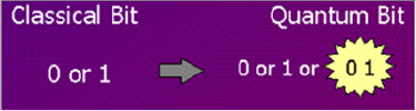
Figure 5: Classical Vs. Quantum Register.

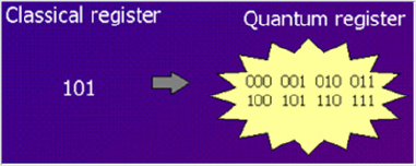
Figure 6: Quantum Processor Demonstration.

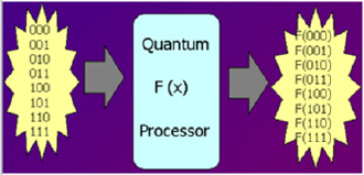
This has impact on the execution time and memory required in the process of computation and determines the efficiency of algorithms. In summary, A memory consisting of N bits of information has 2N possible states. A vector representing all memory states thus has 2N entries (one for each state). This vector is viewed as a probability vector and represents the fact that the memory is to be found in a particular state level. [9]In the classical view, one entry would have a value of 1 (i.e., a 100% probability of being in this state), and all other entries would be zero. In quantum mechanics, probability vectors are generalized to density operators [10]. This is the technically rigorous mathematical foundation for quantum logic gates [11], but the intermediate quantum state vector formalism is usually introduced first because it is conceptually simpler.However, one question arises about Qubits and that is “Why are qubits so fragile?” and here is what we can say.The reality is that the coins, or qubits, eventually stop spinning and collapse into a particular state, whether it’s heads or tails. The goal with quantum computing is to keep them spinning in the superposition of multiple Furthermore, expanding on Quantum Operations, and we stated concerning this operation, the prevailing model of Quantum Computation (QC) describes the computation in terms of a network of Quantum Logic Gates[12].

Bear in mind that, a quantum computing and specifically the quantum circuit model of computation, a quantum logic gate (or merely quantum gate) is a primary quantum circuit operating on a small number of qubits. They are the building blocks of quantum circuits like classical logic gates are for conventional digital circuits [13].States for a long time. Imagine I have a coin spinning on a table, and someone is shaking that table. That might cause the coin to fall over faster. Noise, temperature change, an electrical fluctuation or vibration-all of these things can disturb a qubit’s operation and cause it to lose its data. One way to stabilize certain types of qubits is to keep them very cold. Our qubits operate in a dilution refrigerator that’s about the size of a 55-gallon drum and use a particular isotope of helium to cool them a fraction of a degree above absolute zero (roughly –273 degrees Celsius) [7].There are probably no less than six or seven different types of qubits, and probably three or four of them are being actively considered for use in quantum computing. The differences are in how you manipulate the qubits, and how you get them to talk to one another. You need two qubits to talk to one another to do large “entangled” calculations, and different qubit types have different ways of entangling.Another approach uses the oscillating charges of trapped ions-held in place in a vacuum chamber by laser beams-to function as qubits. Intel is not developing trapped ion systems because they require a deep knowledge of lasers and optics, which is not necessarily suited to our strengths.Furthermore, quantum computers being built by Google, IBM, and others. Another approach uses the oscillating charges of trapped ions-held in place in a vacuum chamber by laser beams-to function as qubits. Intel is not developing trapped ion systems because they require a deep knowledge of lasers and optics, which is not necessarily suited to our strengths.

How Powerful Are Quantum Computers?

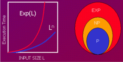
For an algorithm to be efficient, the time it will take to execute the algorithm must increase not faster than a Polynomial Function of the size of the input. For example, let us think about the input size as the total number of bits needed to specify the input to the problem, as demonstrated in(Figure 7). The number of bits required to encode the number we want to factorize is an example of this scenario.If the best algorithm we know for a particular problem has the execution time, which can be viewed as a function of the size of the input, bounded by a polynomial, then we say that the problem belongs to Class P, as it is shown in (Figure 7).Problems outside class P are known as hard problems. Thus, we say, for example, that multiplication is in P, whereas factorization is not in P. “Hard” in this case does not mean that it is “impossible to solve” or “noncomputable”. It means that the physical resources needed to factor a large number scale up such that, for all practical purposes, it can be regarded as intractable.However, some quantum algorithms can turn hard mathematical problems into easy ones – factoring being the most striking example as far as we are concerned so far. Such a scenario can be seen in cryptographic technology to be able to decipher a code of cryptic streams or communications. One can see a huge application of it in Rivest, Shamir, and Adelman (RSA) Data Security[8].

Figure 7: Polynomial Function.

The difficulty of factorization underpins the security of what are currently the most trusted methods of public-key encryption, in particular of the RSA system, which is often used to protect electronic bank account, as depicted in (Figure 8).Once a quantum factorization engine, which is a special-purpose quantum computer for a factorizing large number, is built, all such cryptographic systems will become insecure, and they will be wide-open for smart malware to pass through the gate of cybersecurity wall of the system under the attack by this malware.The potential use of quantum factoring for code-breaking purposes has raised the apparent suggestion of building a Quantum Computer (QC), however this not the only application QC. With signs of progress in the utilization of Artificial Intelligence (AI) in the recent decade and pushing toward Super Artificial Intelligence (SAI) to deal with massive sheer of data at Big Data (BD) volume, a need for Quantum Computing versus Classical Computing is felt by the today’s market standard.A supervised AI or SAI with an integrated element of Machine Learning (ML) and Deep Learning (DL) allows us to prosses all of the historical data by comparing them with a collection of incoming data via DL and ML to collect the right information for a proper decision making of the ongoing day-to-day operation and most importantly to be able to forecast future as a paradigm model [14-17].

Figure 8: RSA Data Security Key.

The impact of quantum computing on developing a better artificial intelligence and its next-generation super artificial intelligence can be seen as ongoing technology efforts by scientists and engineers as a common denominator.Typically, the first quantum algorithms that get proposed are for security (such as cryptography) or chemistry and materials modeling. These are problems that are essentially intractable with conventional computers. That said, there are a host of papers as well as start-up companies and university groups working on things like machine learning and AI using quantum computers. Given the time frame for AI development, “I would expect conventional chips optimized specifically for AI algorithms to have more of an impact on the technology than quantum chips,” says Jim Clarke, Intel’s Head of Quantum Computing. Still, AI is undoubtedly a fair game for quantum computing.

How to Build Quantum Computers?

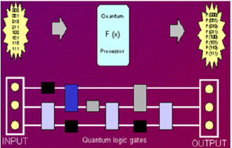
In principle, engines know, how to build a Quantum Computer; we start with simple quantum logic gates as it was described in general previously and connect them up into quantum networks [9] as depicted herein (Figure 9).A Quantum Logic Gate (QLG), like its cousin Classical Logic Gate (CLG), is a straightforward computing device that performs one elementary quantum operation around qubit, usually on two qubits, in a given time. Of course, quantum logic gates differ from their classical counterparts in that they can create and perform operations on quantum superposition as we stated before.As the number of quantum gates in a network increases, we quickly run into some serious practical problems. The more interacting qubits are involved, the harder it tends to be engineering the interaction that would display the quantum properties.The more components there are, the more likely it is that quantum information will spread outside the quantum computer and be lost into the environment, thus spoiling the computation. This process is called decoherence. Therefore, our task is to engineer a sub-microscopic system in which qubits affect each other but not the environment.This usually means isolating the system from its environment as interactions with the external world cause the system to decohere. However, other sources of decoherence also exist. Examples include the quantum gates, and the lattice vibrations and background thermonuclear spin of the physical system used to implement the qubits. Decoherence is irreversible, as it is effectively non-unitary, and is usually something that should be highly controlled, if not avoided.

Figure 9: A Simple Quantum Logic Gates.

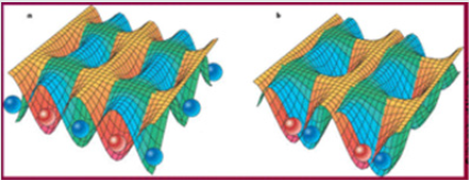
Considering such constraint, then it is clear which technology will support quantum computation going forward in the future of this technology. Today simple quantum logic gates involving two qubits, as we said, are being realized and recognized in laboratories as stepping forward. Current experiments range from trapped ions via atoms in an array of potential wells created by a pattern of the crossed laser beam to electrons in semiconductors. See (Figure 10) However, the technology of the next decade should bring control over several qubits and, without any doubt, we shall already begin to benefit from our new way of harnessing nature.There are several models of quantum computing, including the quantum circuit model, quantum Turing machine, adiabatic quantum computer, one-way quantum computer, and various quantum cellular automata. The most widely used model is the quantum circuit. Quantum circuits are based on the quantum bit, or “qubit”, which is somewhat analogous to the bit in classical computation. Qubits can be in a 1 or 0 quantum state, or they can be in a superposition of the 1 and 0 states. However, when qubits are measured, the result is always either a 0 or a 1; the probabilities of these two outcomes depend on the quantum state that they were in immediately before the measurement. Computation is performed by manipulating qubits with quantum logic gates, which are somewhat analogous to classical logic gates[9].There are currently two main approaches to physically implementing a quantum computer: analog and digital. Analog methods are further divided into the quantum simulation, quantum annealing, and adiabatic quantum computation. Digital quantum computers use quantum logic gates to do computation. Both approaches use quantum bits or qubits[10] There are currently several significant obstacles in the way of constructing useful quantum computers. In particular, it is difficult to maintain the quantum states of qubits as they are prone to quantum decoherence, and quantum computers require significant error correction as they are far more prone to errors than classical computers[10].

Figure 10: Patten of Crossed Laser Beam.

Conclusion

The race is on to build the world’s first meaningful quantum computer-one that can deliver the technology’s long-promised ability to help scientists do things like develop miraculous new materials, encrypt data with near-perfect security and accurately predict how Earth’s climate will change. Such a machine is likely more than a decade away, but IBM, Microsoft, Google, Intel, and other tech heavyweights breathlessly tout each tiny, incremental step along the way. Most of these milestones involve packing more quantum bits, or qubits-the basic unit of information in a quantum computer-onto a processor chip ever. But the path to quantum computing involves far more than wrangling subatomic particles. However, the question of “When will we see working Quantum Computer solving real-world problems?” remains to be answered. The first transistor was introduced in 1947. The first integrated circuit followed in 1958. Intel’s first microprocessor-which had only about 2,500 transistors-didn’t arrive until 1971. Each of those milestones was more than a decade apart. People think quantum computers are just around the corner, but history shows these advances take time. If 10 years from now we have a quantum computer that has a few thousand qubits, that would undoubtedly change the world in the same way the first microprocessor did. We and others have been saying it’s ten years away. Some are saying it’s just three years away, and I would argue that they don’t have an understanding of how complex the technology is.
At the end, it is worthy to say that “Any computational problem that can be solved by a classical computer can also, in principle, be solved by a quantum computer. Conversely, quantum computers obey the Church–Turing thesis; that is, any computational problem that can be solved by a quantum computer can also be solved by a classical computer. While this means that quantum computers provide no additional power over classical computers in terms of computability, they do, in theory, provide extra power when it comes to the time complexity of solving certain problems.Notably, quantum computers are believed to be able to quickly solve certain problems that no classical computer could solve in any feasible amount of time-a feat known as “quantum supremacy” [10].The study of the computational complexity of problems concerning quantum computers is known as quantum complexity theory.

For more Lupine Publishers Open Access Journals Please visit our website:

 wt u have given that link add For more Modern Approaches on Material Science articles Please Click Here:

https://lupinepublishers.com/material-science-journal/

Lupine Publishers| An Alternative Strategy for the Use of a Low-Cost, Age- Hard enable Fe-Si-Ti Steel for Automotive Application

 Lupine Publishers| Modern Approaches On Material Science

Abstract

For High Strength Low Alloy (HSLA) steels or for age-hard enable steels (miraging) the strengthening by precipitation is done before forming operation to increase the yield stress as much as possible. In this publication the advantages of a hardening thermal treatment after forming operation are investigated in a low-cost age-hard enable steel Fe-Si-Ti consistent with automotive application.

Keywords: Age-hard enable, Precipitation, Forming, Ductility

Introduction

The high strength low alloy (HSLA) steels are a group of low carbon steels with small amounts of alloying elements (as Ti, V, Nb, etc.) to obtain a good combination of strength, toughness, and weldability [1-3]. By the addition of micro-alloying elements (less than 0.5 wt.%), HSLA steels are strengthened by grain refinement strengthening, solid solution strengthening and precipitation hardening [4-8]. Regarding automotive applications, the entire range of HSLA steels are suitable for structural components of cars, trucks, and trailers such as suspension systems, chassis, and reinforcement parts. HSLA steels offer good fatigue and impact strengths. Given these characteristics, this class of steels offers weight reduction for reinforcement and structural components [9-11]. Despite the interest of HSLA, the precipitation hardening is about 100MPa. So the new targets concerning the CO₂ emission of vehicles push the steel-makers to develop Advanced High Strength Steels (Dual-Phase, Transformation Induced Plasticity) hardened by multiphase microstructures containing 10 to 100% of martensite [12] which offer a better combination between strength and ductility for an acceptable cost Let’s notice that the Ultimate Tensile Strength (UTS) increases more that the Yield Stress (YS). YS is crucial for anti-intrusive aspect during a crash [12]. In the other side, because there is no phase transformation in Aluminum, age-hardening by precipitation is widely used in Aluminium alloys hardened by various additive elements [see [13] for a review]. The volume fraction of precipitates is several percent’s, the hardening can be increased up to 400MPa, but the ductility decreases rapidly.
In steel, there is only miraging steels which are strengthened by a massive precipitation of a martensitic matrix [see [14] for a review]. Despite the impressive YS (up to 2.5GPa), the uniform elongation is less than 1%. Consequently, no forming operation is possible. In addition, the high contents of nickel (about 18%), of molybdenum and of cobalt make these steels very expensive and so they are never used in automotive industry. On the contrary, in the 60’s authors investigated other kind of steels suitable to be strongly hardened by massive intermetallic precipitation without extracost [15,16]. Among the different investigated system, the Fe-Si-Ti alloys are the most promising. This is the reason why a series of publications has been dedicated to this system in the 70’s by Jack&al. [17-19]. Unfortunately, hardness and compression behaviour have been only reported and a lot of discussions concerned the nature of the precipitates (Fe₂Ti, FeSi, or Fe2SiTi) have been reported. More recently a systematic study of precipitation kinetics in a Fe_-2.5%Si- 1%Ti alloy in the temperature range 723 K to 853 K (450°C to 580°C), combining complementary tools transmission electron microscopy (TEM), atom probe tomography (APT), and Small-Angle-Neutron Scattering (SANS)) have been carried out [20]. It has been shown that the Heusler phase Fe2SiTi dominates the precipitation process in the investigated time and temperature range, regardless of the details of the initial temperature history.

Figure 1: Summary of the different strategies for the use of precipitation hardened steels: The green arrow is the usual one, the orange is the strategy developed in this publication.

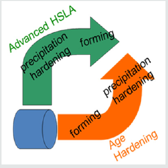
Considering that the ductility decreases regularly as a function of the hardening up to 1.2GPa and because it is targeted to obtain a steel suitable for deep drawing the strategy showed in (Figure 1). (orange arrow) has been investigated. The objective is to form a material as soft as possible and as ductile as possible and to obtain the hardening by a thermal treatment after forming. This publication presents the characterization of this way to manage the situation. It is noticed that as Si and Ti promote ferrite, there is no phase transformation whatever the thermal treatment. (Figure 1) Summary of the different strategies for the use of precipitation hardened steels: The green arrow is the usual one, the orange is the strategy developed in this publication.

Results

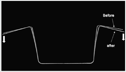
In order to assess for the first time in steel for automotive applications, the hardening have been chosen followed a thermal treatment at 500°C for two hours consistent with the kinetic determined by SANS [20]. As shown in (Figure 2). illustrating the tensile behavior of the steel consisting only in solid solution (i.e. only after recrystallization) is very ductile as for IF steels but with a higher yield stress due to solid solution hardening. After treatment and hardening of 300MPa is obtained with promising ductility. As shown in (Figure 3) the treatment has induced the expected massive precipitation of Fe2SiTi (3.8% weight percent with a radius of 4nm determined by TEM and SANS [20]). To assess the metallurgical route, the (Figure 4). shows that it is possible to severely bend the steel consisting only in solid solution without any defect up to an angle of 180°. Hardness trough the thickness has been measured before and after the thermal treatment (Figure 5). The value confirms the hardening by precipitation. It is noticed that tis precipitation hardening is not sensitive to the strain hardening induced by bending trough the thickness. Because the alloy is dedicated to automotive industry, the drawing must be investigated. This the reason why a cup obtained by deep drawing of 5cm diameter has been manufactured using the steel consisting in solid solution without any problem as illustrated in (Figure 6). It confirms the very high ductility before heat treatment. One another problem in automotive industry is the increase in spring-back with an increase in strength. In addition, it is very difficult to predict or to model this phenomenon. As shown in (Figure 7). this aspect has been studied by a standard test base the forming of a hat-shaped part. It is highlighted that the spring-back during the treatment is weak. That is probably because there is no phase transformation during precipitation and so no internal stresses.

Figure 2: Tensile curves before and after the ageing treatment.

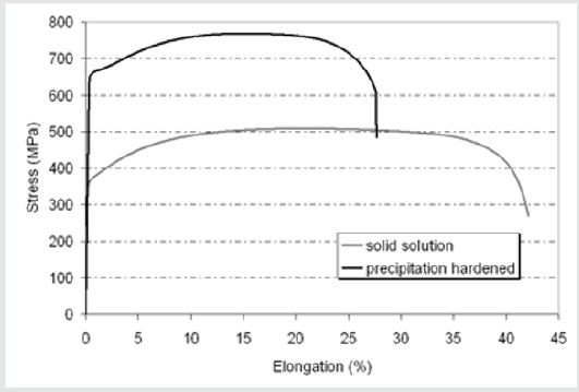
Figure 3: TEM micrography showing the massive precipitation of Fe₂SiTi after 2 hours at 500°C (the composition have been determined by APT [20]).

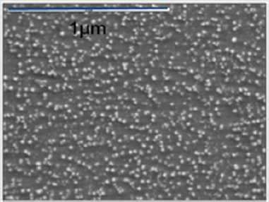
Figure 4: Fully bent specimen before heat treatment (bending angle of 180°).

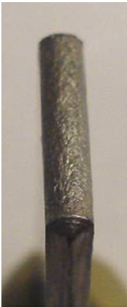
Figure 5: Hardness measurement trough the thickness of the fully bent specimen (i.e. angle of 180°) before and after heat treatment.

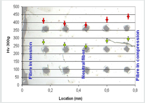
Figure 6: Cup drawing before the hardening heat treatment (5cm diameter).

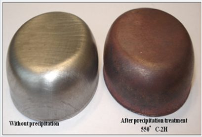
Figure 7: Evaluation of the effect of heat treatment on the spring-back.

Conclusion

For the first time in steel industry for automotive industry a low cost age-hard enable steel has been studied following a strategy based on forming operations before the heat treatment. The bending, the drawability and the spring-back have been investigated highlighting promising results. In addition, the alloy exhibits a cost acceptable for automotive industry. In the future crashworthiness and weldability should be assessed after heat treatment. One of the last advantages is that a lot of parts can be treated at the same time in a furnace usually dedicated to tempering treatment.

For more Lupine Publishers Open Access Journals Please visit our website:

 wt u have given that link add For more Modern Approaches on Material Science articles Please Click Here:

https://lupinepublishers.com/material-science-journal/

Lupine Publishers| Monitoring Time-Progression of Structural, Magnetic Properties of Ni Nano Ferrite During Synthesis

 Lupine Publishers| Modern Approaches On Material Science

Abstract

We present time-progression of structural, magnetic properties of NiFe₂O₄ nano ferrite during its synthesis via sol-gel auto combustion technique, monitored by x-ray diffraction XRD, and magnetic measurements. XRD patterns of the samples collected between 18-52 minutes shows the formation of the nano spinel phase (grain diameter: 15.4 nm-28.6 nm), presence of a-Fe2O₃phase was also detected. Samples collected between 8-14 minutes show the amorphous nature of the samples. Time-progression studies show: a) sample taken after 20 minutes shows a sharp decrease of specific surface area (range between 39.01 m²/g to 72.73 m²/g), b) non-equilibrium cationic distribution for samples taken between 16-20 minutes with a continuous increase of Fe³⁺ ions population on B-site with simultaneous decrease of Ni²⁺ population, c) for samples taken after 22, 52 minutes, cationic distribution is close to its ideal value of (Fe³⁺) [Ni²⁺Fe³⁺], d) alteration of a degree of inversion (d), oxygen parameter (u), modification of A-O-B, A-O-A, B-O-B super-exchange interactions, e) ferrimagnetically aligned core, and spin disorder on the surface with a thickness between 1.9 nm to 3.6 nm, reducing the saturation magnetization (ranging between 11.7 - 25.5 Am²/kg), as compared to bulk Ni ferrite (55 Am²/kg), f) low squareness ratio values (0.15-0.22) shows the presence of multi-domain nanoparticles, with coercivity between 111-157 Oe.

Keywords: Time-evolution of properties; Sol-gel auto combustion synthesis; XRD; Nano Ni ferrite; Cationic distribution; Magnetic properties

Introduction

Spinel ferrites with general formula Me²⁺O.Fe³⁺₂ O₃, [Me: Divalent metal ion e.g. – Ni²⁺, Zn²⁺, Mg²⁺ Co²⁺ etc.], display face-centered cubic (fcc) structure, with two inter-penetrating sub-lattices: tetrahedrally coordinated (A site), octahedrally coordinated (B site) [1]. Nickel ferrite (NiFe₂O₄) has inverse spinel structure expressed as: (Fe³⁺) [Ni²⁺Fe³⁺] [1]. Allocation of cations on A, B site is crucial in determining properties of spinel ferrites [2,3], can be effectively used to achieve desired properties. Literature gives Ni ferrite synthesis using various methods including mechanical milling [4], coprecipitation [5], hydrothermal synthesis [6], sol-gel auto combustion method [7], showing the effect of the technique on structural, magnetic properties. Literature also reports real-time monitoring (in-situ studies) of properties [8,9], require special, sophisticated equipment, may not be available in all laboratories. Ex-situ monitoring of properties [10], describing the time-evolution of structural, magnetic properties, is a rather simple, more convenient way to perform experiments by utilizing standard laboratory equipment available in many laboratories. Ni ferrite is used in magnetic resonance imaging (MRI) agents [5], photocatalysis for water purification, antimicrobial activity [11], etc.) hence tuning its properties are preferred for improved efficiency.So, in this work, we present the time-development of structural, magnetic properties of NiFe₂O₄ nano ferrite during its synthesis via sol-gel auto combustion technique. Prepared samples are investigated via x-ray diffraction 'XRD,' vibration sample magnetometry, to get complimentary information on structural, magnetic properties.

Experimental Details

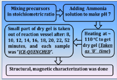
NiFe₂O₄ ferrite samples were synthesized by the sol-gel auto-combustion protocol, as described in detail in [12], by utilizing AR grade -nitrate/acetate-citrate precursors: Nickel acetate - Ni(CH₃CO₂)₂·4H₂O, Ferric nitrate (Fe(NO₃)₃.9H₂O), Citric acid - C₆H₈O₇]. The precursors were mixed in the stoichiometric ratio, were dissolved in 10 ml de-ionized water by keeping metal salts to fuel (citric acid) ratio as 1:1. At the same time, the solution pH was maintained at 7. Now the solution was heated at ~110 ̊C. As dry gel starts to form (taken as 0 minutes) small part of the sample is taken out from the reaction vessel (in an interval of 8, 10, 12, 14, 16, 18, 22, and 52 minutes), and were immediately ice-quenched to room temperature. Powder samples were used for Cu-K- X-ray diffraction 'XRD' measurements (Bruker D8 diffractometer), hysteresis loops by vibrating sample magnetometer. Full-profile XRD analysis was done by MAUD Rietveld refinement software [13] to obtain the lattice parameter (apex.). XRD analysis gives Scherrer's crystalline size D (calculated by the integral width of 311 peak, corrected for instrumental broadening), specific surface area (S), inversion parameter (d), oxygen parameter (u). XRD data was also analysed to get cationic distribution via Bertaut method [14], This provides cationic distribution by comparing experimental and computed intensity ratio of planes I(220)/I(400) and I(400)/I(422), susceptible to cationic distribution [12]. Cationic distribution was used to calculate theoretical or Néel magnetic moment at 0K (Ms(th)), theoretical lattice parameter (ath.), bond angles (θ₁, θ₂, θ₃, θ₄, θ₅) as shown in [3]. Coercivity (Hc), saturation magnetization (Ms), remanence (Mr), squareness ratio (Mr/Ms) was obtained from hysteresis loops. (Figure 1) gives the schematic of sample synthesis and characterization.

Figure 1: Schematic of sample synthesis and characterization.

Results and Discussion

(Figure 2) (a) gives XRD-patterns of the studied NiFe₂O₄ samples collected after 18, 20, 22, and 52 minutes, confirm the formation of the spinel phase. XRD patterns also show the presence of a-Fe2O3 phase, ascribable to sample synthesis at a reasonably lower temperature (~110̊C), as reported in [15], while its disappearance is seen after higher sintering temperature. Figure 1(a) inset shows XRD patterns of samples collected after 8, 10, 12, 14 minutes show the amorphous nature of the samples. Only in the sample collected after 14 minutes, there is the start of spinel phase formation (indicated by a dotted circle). Illustrative Rietveld refined XRD pattern (Figure 2) b) of NiFe₂O₄ sample taken after 20 minutes also validates the cubic spinel ferrite phase formation. (Figure 2)(c) shows a variation of D (range between 15.4 nm to 28.6 nm) and S (range between 39.01 m²/g to 72.73 m²/g) for NiFe₂O₄ samples taken after 16, 18, 20 22, 52 minutes. A perusal of (Figure 2) (c) shows a well-known inverse relationship shown by the expression: [S = [6/(D ´r_XRD)], where r_XRDis x-ray density, as was also reported in[2]. (Figure 2) (c) shows that for samples taken after 22, 52 minutes, D sharply increases with concurrent reduction of S, is ascribable to significant changes in cationic distribution via migration of Ni²⁺ions to B site with simultaneous migration of Fe³⁺ ions on A site(as can be seen in Table 1). (Figure 2 )(c) inset display linear relation between d and u as was also observed earlier [3], shows that reduction of the degree of inversion (d) leads to a reduction of oxygen parameter (u), a measure of disorder in the studied system, is expected to affect the properties of the studied samples. Table 1 depicts the variation of experimental and theoretical lattice parameter (a_exp., a_th. ), inversion parameter (d), oxygen parameter (u), Cation distribution (for A, B site), and calculated, observed intensity ratios for I400/422, I220/400 plane for the studied samples. The observed variation of a_exp. is consistent with changes in cationic distribution, and variation of the degree of inversion (d). Close agreement between observed, calculated a_exp., a_th. suggests that the computed cationic distribution agrees well with real distribution [16]. Close matching of calculated, observed intensity ratios for I400/422, I220/400 signifies an accurate cationic distribution among A, B site [17]. Cationic distribution illustrates that as we go from NiFe₂O₄ samples taken after 16, 18, and 20 minutes, the population of Fe³⁺ ions on B site increases from 1.2 to 1.5 with a concurrent decrease of Ni²⁺ ions from 0.80 to 0.50. For samples taken after 22, 52 minutes Fe³⁺ population on B site decreases, while Ni²⁺ ion population increases up to 0.98, which is close to the ideal inverse cationic distribution of (Fe³⁺) [Ni²⁺Fe³⁺] [1].

Figure 2: (a): XRD patterns of the studied NiFe₂O₄ samples taken after 16, 18, 20 22, 52 minutes showing the formation of the spinel phase. Inset: XRD patterns of the studied samples taken after 8, 10, 12, 14 minutes. (b): Illustrative Rietveld refined XRD pattern of NiFe₂O₄ sample taken after 20 minutes (* - Experimental data, Solid line - theoretically analyzed data, |- Bragg peak positions, Bottom line- Difference between experimental, and fitted data). (c) variation of grain diameter (D) and specific surface area (S) for NiFe₂O₄samples taken after 16, 18, 20 22, 52 minutes. Line connecting points guide to the eye. Inset: variation of inversion parameter (d) with oxygen parameter (u). The straight line is a linear fit to the experimental data.

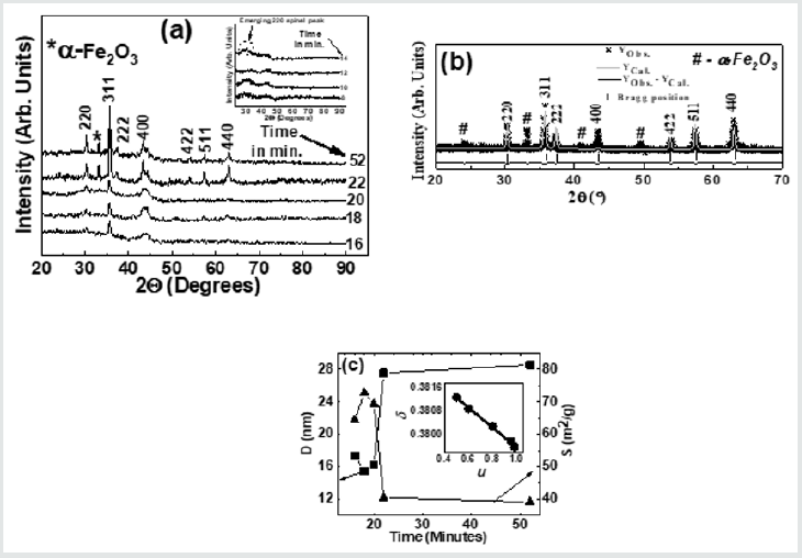
Figure 3 depicts the variation of bond angles between cations, cation-anion q₁, q_2,q₃, q₄and q₅, for the studied samples taken between 16 - 52 minutes. In samples taken after 8, 10, 12, and 14 minutes, due to the absence of the spinel phase, bond angles could not be computed. Bond angles provide information on super-exchange interaction (A-O-B, A-O-A, B-O-B), mediate by oxygen. (Figure 3) shows that for samples taken after 16, 16, 20 minutes q₁, q₂, q₅, decreases while q₃, q₄increases, indicates a weakening of A–O–B, A– O–A and strengthening B–O–B super-exchange interaction as is also observed earlier [16]. For samples taken after 22, 52 minutes q₁, q₂, q₅, increases, and q₃, q₄decreases reveals strengthening of A-O-B, A-O-A, and weakening of B-O-B super-exchange interaction, reported in the literature with compositional changes [3]. Samples taken after different times, there is a modification of A-O-B, A-O-A, B-O-B super-exchange interactions, are attributed to changes in dand u as shown in(Table 1), observed with compositional changes [3,16]. Observed A-O-B, A-O-A, B-O-B super-exchange interactions should mirror in magnetic properties, matches well with reported literature [3,16]. Thus, collecting samples after different times during synthesis is analogous to compositional changes in spinel ferrites, affects structural, magnetic properties [3, 12, 16, 18].

Figure 3: Dependence of bond angles (q₁^A-O-B,q₂^A-O-B, q₃^B-O-B,q₄^B-O-B, q₅^A-O-A) for NiFe₂O₄ samples taken after 16, 18, 20 22, 52 minutes. Line connecting points guide to the eye.

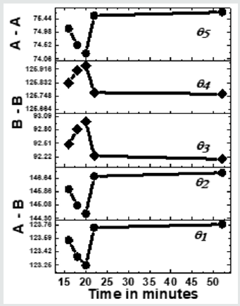
Figure 4 depicts hysteresis loops, reveal changes in Ms_(exp.)samples taken after 16, 18, 20 22, 52 minutes, attributable to alteration of B-O-B, A-O-B, and A-O-A interaction, depends on bond angles, as shown in (Figure 3), and cationic distribution, as shown in (Table 1). (Figure 4) inset displays hysteresis loops of the samples taken after 8, 10, 12, 14 minutes, showing very low magnetization, attributable to the fact that in these samples ferrite phase is not formed, as was also observed in XRD data shown inset of (Figure 2) (a). Observed lower values of M_s(exp.) (ranging between 11.7 - 25.5 Am²/kg) as compared to the multi-domain bulk Ni ferrite (55 Am²/kg) is attributed to the two-component nanoparticle system as described in [19]consisting of a spin-disorder on the surface layer and ferrimagnetically aligned spins within the core. Computed magnetic dead layer thickness as described in [20,21]for NiFe₂O₄ samples taken after 16, 18, 20 22, 52 minutes are respectively 2.3, 1.8, 1.9, 2.5 and 3.6 nm. They confirm the contribution of 'dead layer thickness' in the reduction of M_s(exp.), apart from B-O-B, A-O-B, and A-O-A super-exchange interaction and cationic distribution.

Figure 4: Hysteresis loops of the studied NiFe₂O₄ samples taken after 16, 18, 20 22, 52 minutes. Inset: Hysteresis loops of the samples taken after 8, 10, 12, 14 minutes.

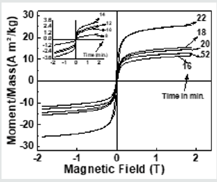
Table 1: Variation of experimental and theoretical lattice parameter (a_exp., a_th.), inversion parameter (), oxygen parameter (u), Cation distribution (for A, B site), and observed, calculated intensity ratios for I400/422, I220/400 plane for the studied samples.

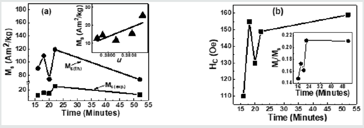
Figure 5(a) depicts Variation of M_s(exp.), M_s(th.)for NiFe₂O₄ samples taken after 16, 18, 20 22, 52 minutes. A perusal of figure 5(a) shows that observed behaviour is attributable to alteration of B-O-B, A-O-B, and A-O-A super-exchange interaction, depends on bond angles (see figure 3), and cationic distribution (see Table 1). Non-similar trend of M_s(exp.), M_s(th.)in (Figure 5)(a), shows that the magnetization behaviour is governed by Yafet-Kittel three sub-lattice model, described in [22], confirmed by the computed canting angle (a_Y-K) values for NiFe₂O₄ samples taken after 16, 18, 20 22, 52 minutes, which are respectively 52.7, 56.6, 46.2, 55.7, 46.9 ̊. The canting angle provides information on spin canting on the surface, is so-called 'magnetic dead layer,' leads to a reduction of M_s(exp.), which is lower than bulk saturation magnetization of Ni ferrite (55 Am²/kg). Inset of Figure 5 (a) shows the variation of M_s(exp.) with oxygen parameter 'u'(which is a measure of disorder in the samples [1]). Figure 5 (a) shows the disorder-induced enhancement of M_s(exp.),as was also reported in [3]. (Figure 5) (b) depicts the Coercivity(H_c) variation for NiFe₂O₄ samples taken after 16, 18, 20 22, 52 minutes. Obtained H_cand related Dvalues imply that studied samples lie in the region with overlap between single or multi-domain structures, as reported earlier [3]. (Figure 5) (b) Inset depicts the variation of Mr/Ms for NiFe₂O₄ samples taken after 16, 18, 20 22, 52 minutes. Mr/Ms values ranging between 0.15-0.22 reveal enhanced inter-grain interactions suggesting isotropic behavior of the material [23] reveal multi-domain particles with no preferential magnetization direction. Time-dependent tunable structural, magnetic properties during synthesis are valuable in achieving optimal properties of Ni ferrite for their usage in magnetic resonance imaging [5], hyperthermia [24] for cancer treatment, photocatalysis for water purification [11].

Figure 5: (a) Variation of M_s(exp.), M_s(th.)for NiFe₂O₄ samples taken after 16, 18, 20 22, 52 minutes. Inset: Dependence of M_s(exp.)on oxygen parameter (u), line connecting points in Inset are linear fit to the experimental data.; (b) Coercivity(H_c) variation for NiFe₂O₄ samples taken after 16, 18, 20 22, 52 minutes. Inset: Variation of M_r/M_sfor NiFe₂O₄ samples taken after 16, 18, 20 22, 52 minutes.

Summary

To summarize, the sol-gel auto combustion technique is used to observe the time-development of structural, magnetic properties of Ni ferrite. Changes in cationic distribution lead to modification of structural properties, magnetic interactions, responsible for observed magnetic properties. Time-progression of properties are of use to alter structural, magnetic properties of Ni ferrite as a material for its prospective usage in heterogeneous catalysis, water purifications, biomedical applications.

Acknowledgments

Authors thank Dr. M. Gupta-L. Behra, UGC-DAE CSR, Indore for XRD measurements. Work supported by UGC-DAE CSR, Indore project (No.: CSR-IC-ISUM-25/CRS-308/2019-20/1360, dated March 5, 2020).

Conflicts of Interest

Author

Author Contributions

Conception: SNK; Sample synthesis, RV, SNK; Measurements, analysis of data: SNK, RV; Supervision, Resources, supervision, project management: SNK; Writing the manuscript: SNK, RV. All authors approve the draft and participate in reviewing.

For more Lupine Publishers Open Access Journals Please visit our website:

 wt u have given that link add For more Modern Approaches on Material Science articles Please Click Here:

https://lupinepublishers.com/material-science-journal/